Workflow Patterns

Most computational studies, whatever their domain, are built from three recurring structures. Recognising them in your own study is the most useful first step in applying the approach, because each pattern pulls in specific recommendations.

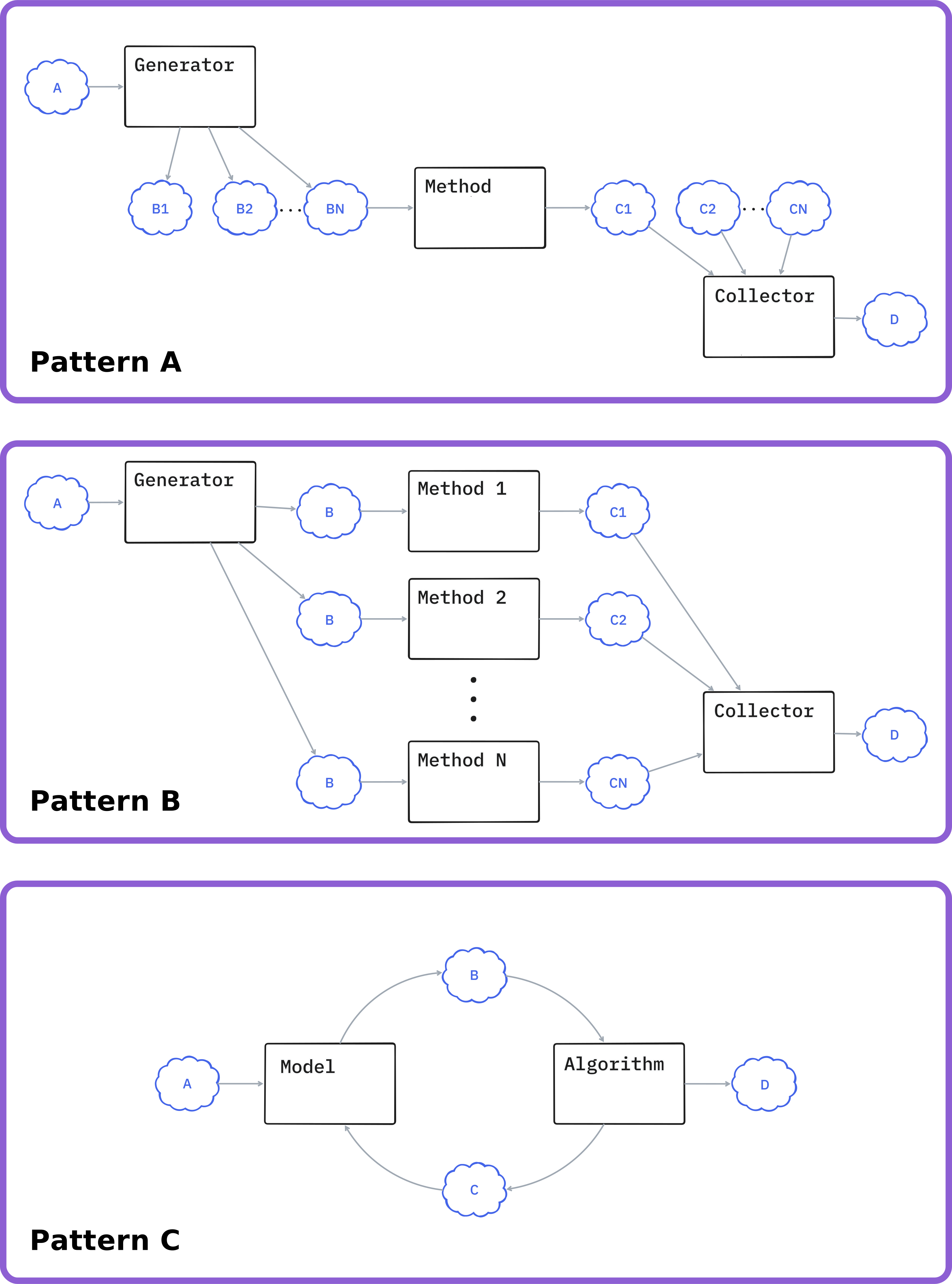
Pattern A: parameter sweep pipeline

One computational unit processes many distinct inputs. A generator produces a large set of input configurations (a parameter sweep, varied initial conditions, sampled designs), each configuration is dispatched independently to the same method, and a collector aggregates the outputs into one dataset.

We meet this pattern when training a surrogate model on simulator runs spread across a parameter space, in Monte Carlo uncertainty propagation, and in Sobol sensitivity analysis, where the collected input-output dataset feeds the computation of sensitivity indices.

Pattern B: fan-out/fan-in pipeline

Many distinct computational units process the same input. A generator produces one shared input, several method implementations each consume it, and a collector gathers the outputs for comparison. The implementations solve the same problem but differ in mathematical formulation, programming language, or both.

This is the shape of method benchmarking, of ensemble runs with different random seeds, and of inference diagnostics where one set of results fans out to complementary analyses that are gathered into a report.

Pattern C: model-based online loop

A model and an algorithm are coupled at run time as a client-server pair. The algorithm queries the model iteratively until an objective is reached, which means both must be alive at the same time. This is fundamentally different from A and B, where every unit starts, runs once, and exits.

Optimisation, Bayesian parameter calibration, model selection, optimal experimental design, and data assimilation all follow this pattern.

Patterns compose

A real study rarely matches exactly one pattern. Patterns nest: the method inside a sweep (Pattern A) or a benchmark (Pattern B) may itself be a model-algorithm loop (Pattern C). A calibration study that sweeps over several experimental datasets is a Pattern A whose method is a Pattern C. A unit may also hide tightly coupled internals, such as an MPI-parallel solver, without changing the pattern around it.

So instead of asking "which pattern is my study?", we decompose it level by level: identify the outermost structure, then look inside each unit for further structure. Every pattern occurrence found this way pulls in its own recommendations.

What each pattern asks for

All three patterns need isolated units (Iso1 onwards) and language-agnostic data at unit boundaries (Int1). Beyond that shared baseline, each pattern has a characteristic emphasis.

Pattern A means many executions of one unit. Automating the sweep (Orch1), scheduling it across available resources (Orch2), and not repeating completed runs after an interruption (Orch3) matter most here.

Pattern B means several independently developed units side by side, often in different languages with conflicting dependencies. Per-unit environments (Iso1, Iso2) keep the implementations from interfering, and a shared boundary format (Int1) lets the collector read every output the same way.

Pattern C means high-frequency data exchange between two live units. That calls for a bandwidth-conscious exchange mechanism (Int3) and for running a unit as a long-lived service under a workflow manager (Orch4), which breaks the assumptions most workflow tools make.

Once you know which recommendations your study touches, the three pillars page gives you the complete map.